Open any image in a hex editor. A photo of a street sign, a receipt, a screenshot of a PDF. At offset zero you get the format header. A few kilobytes in, you hit the pixel data: three bytes per pixel in RGB, a grid of numbers where (128, 52, 19) might be a brick wall and (240, 238, 220) might be paper. Somewhere in that grid sits a stop sign with the word "STOP" rendered in white Highway Gothic on red. A human sees four letters. The computer sees a 47 × 19 patch of red-adjacent pixel values where the R channel hovers near 200 and G and B dip below 40. Mapping that patch to the string "STOP" is optical character recognition, and it has been an open research problem since Gustav Tauschek patented the first reading machine in 1929.
OCR is deceptively hard because reading is deceptively easy. A six-year-old can recognize the letter A in a dozen fonts, at multiple sizes, under uneven lighting, slightly rotated, partially occluded, and written in pencil. A computer needs a pipeline: clean the image, find the text regions, segment the characters or glyph sequences, and classify each one. Each of those stages has a failure mode, and the failures compound.
What makes OCR hard
The core problem is not classification. Classifying a pre-segmented 28 × 28 character image into one of 62 classes (A–Z, a–z, 0–9) is a task a 1990s LeNet can solve at 99% accuracy. The hard part is everything that comes before the classifier.
Font variation. The letter "g" has at least four common structural variants: single-story ( handwritten ), double-story ( most serif faces ), the loop-tail found in Helvetica, and the open-tail in Futura. A model trained on Tahoma will misread Univers at a measurable rate. Real-world OCR covers hundreds of typefaces plus handwriting, which has no consistent stroke topology at all.
Geometric distortion. Photos of documents are rarely flatbed scans. A phone photo of a receipt introduces perspective skew, curvature, and non-uniform scale. Text near the spine of a book bends. Whiteboard photos catch the photographer's shadow. A 10-degree skew reduces Tesseract's accuracy from ~97% to below 85% on standard benchmarks. Deskewing algorithms (Hough line detection, Radon transform, projection profile analysis) recover some of that loss, but none recover all of it.
Illumination and noise. Uneven lighting turns a uniform background into a gradient, breaking global thresholding. JPEG compression artifacts create ringing around sharp edges. In OCR terms, that means ringing around letter strokes. Salt-and-pepper noise from low-light sensors fills white space with dark pixels that look like punctuation. A photocopy of a photocopy smears thin strokes together, merging "rn" into "m" and "cl" into "d."
Layout complexity. Documents have columns, captions, tables, headers, footnotes, and sidebars. Text flows around images. Some languages run right-to-left. Others mix directions in the same paragraph. Identifying reading order (which block of text comes after which) is a layout analysis problem separate from recognition, and getting it wrong scrambles the output even when every character is classified correctly.
Contextual ambiguity. Given only the pixel pattern, "0" (digit zero), "O" (uppercase letter O), and "o" (lowercase letter o) are identical in many sans-serif fonts. "1", "l", "I", and "|" share a vertical stroke. Resolution adds another dimension: at 12 pixels tall, "e" and "c" differ by a single horizontal stroke three pixels wide. Human readers resolve these from context. Machines need language models, statistical or learned, to make the same call.
The traditional OCR pipeline
Before deep learning, OCR was a sequence of hand-designed stages. Each stage was independently developed, often by different research groups, and tuned for a specific degradation. The pipeline looked like this:
Raw image → Preprocessing → Binarization → Deskew → Layout Analysis
  → Character Segmentation → Feature Extraction → Classification
  → Post-processing (language model) → Text output
Preprocessing and binarization
Color images are converted to grayscale. Noise reduction smooths the signal before thresholding. Median filtering handles salt-and-pepper noise. Gaussian blur handles sensor noise. Bilateral filtering is used when edge preservation matters.
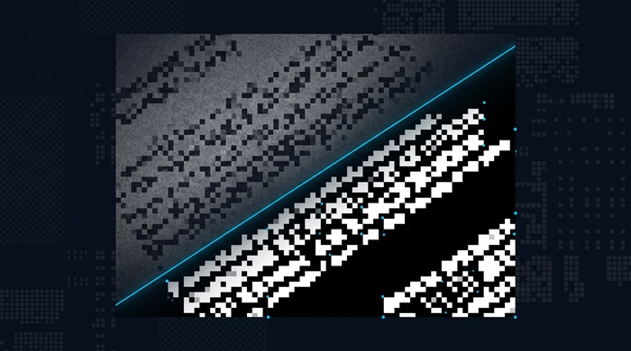
Binarization turns the grayscale image into black text on white background. The standard algorithm is Otsu's method (1979): it exhaustively searches for the threshold that minimizes intra-class variance between foreground and background pixel distributions. Otsu assumes a bimodal histogram (text pixels cluster at one intensity, background pixels at another), which works for flatbed scans under controlled lighting and fails for phone photos with shadows. Local adaptive methods (Sauvola, Niblack) compute a different threshold per pixel based on neighborhood statistics, handling uneven illumination at the cost of artifacts near edges.
Deskew and layout analysis
Document skew is detected by finding lines: either Hough transform on edge pixels, or projection profile analysis where the document is rotated through a range of angles and the angle with the sharpest horizontal projection peaks is chosen. Once the skew angle is known, an affine transform rotates the image back.
Layout analysis segments the page into text blocks. The classic approach runs connected-component analysis (CCA) to find blobs of foreground pixels, groups them into words by proximity, then groups words into lines and lines into blocks. The XY-cut algorithm recursively splits the page by finding whitespace gaps along horizontal and vertical projections, building a tree of regions. Modern implementations use a hybrid: CCA for initial blobs, then a learned model to classify each blob as text, image, table, or separator.
Character segmentation
For machine-printed text, segmentation means cutting word images into individual characters. The vertical projection profile (a histogram of foreground pixel counts per column) produces peaks at character centers and valleys at character boundaries. This works until two characters touch, or one character contains disconnected parts ("i", "j", ":", "%"). Over-segmentation (cutting too aggressively) followed by merging based on classifier confidence is one fix. Another is to skip segmentation entirely and recognize entire words, which is what modern sequence-based methods do.
Feature extraction and classification
Once you have a character image, you need to describe it numerically for a classifier. Pre-deep-learning features included:
- Raw pixel values as a flattened vector (simple, fragile to translation and scale)
- Zoning: divide the character bounding box into an N × N grid, count foreground pixels per cell, use the counts as features
- Gradient-based features (HOG): histogram of oriented gradients captures edge directions, robust to small translations
- Scale-invariant feature transform (SIFT): detects and describes keypoints invariant to scale, rotation, and illumination
The classifier was typically a support vector machine (SVM) with an RBF kernel, trained on tens of thousands of labeled character images per font. A well-tuned SVM + HOG pipeline could hit ~98% per-character accuracy on clean printed text. Drop noisy, skewed, or handwritten input into the same pipeline, and accuracy fell to 70–80%.
Tesseract: from HP Labs to LSTM
Tesseract is the reference open-source OCR engine. It began as a PhD project at HP Labs Bristol in the 1980s, was open-sourced in 2005, and has been maintained by Google since 2006. Its architecture split cleanly into two eras.
Version 3: the classic pipeline
Tesseract 3 implemented the traditional pipeline with a few innovations. Its layout analysis used a tab-stop detection algorithm that found column boundaries by aligning word bounding boxes, a pragmatic heuristic tuned for the kind of documents HP was scanning in the 1990s. Character segmentation used chopper/associator logic: the chopper over-segmented the word image into candidate cuts, and the associator used classifier confidence and a dictionary to decide which cuts to merge.
The classifier was a two-pass system. The first pass (static classifier) matched segmented blobs to prototypes (clustered training samples) using a nearest-neighbor search. The second pass (adaptive classifier) fine-tuned on the document itself, learning the specific font used in that image. The adaptive classifier needed roughly a page of text to become effective, which is why Tesseract 3 performed poorly on single-word images like street signs and captions.
Tesseract 3 shipped .traineddata files: archives containing the prototype clusters, character set definitions, a word-frequency dictionary, and a unichar ambiguity table mapping confusable character pairs. Training a new language required feeding Tesseract images of text paired with ground-truth transcriptions, boxing each character, and running the training tools. A multi-hour process per language.
Version 4/5: LSTM replaces the pipeline
Tesseract 4 (2018) replaced the entire recognition path with a single LSTM neural network. The LSTM operates on a sequence of vertical slices of the text line image, each slice one pixel wide and the full text-line height. Each slice is fed into a stack of bidirectional LSTM layers. The output is a sequence of character probabilities with a Connectionist Temporal Classification (CTC) loss that aligns the variable-length output sequence to the ground-truth text without requiring pre-segmented character positions.
The LSTM model handles variable-width characters, touching characters, and font variation without the chopper/associator machinery. It still relies on Tesseract's legacy layout analysis for finding text lines, but the line recognition is end-to-end neural. On the ICDAR 2017 benchmark, Tesseract 4 achieved 4.4% character error rate (CER) on printed English, compared to 7.2% for Tesseract 3. The training process switched from the legacy boxing tool to combining text lines with transcriptions. Still supervised, but with one label per line instead of per character.
The .traineddata format was extended to hold the LSTM model weights (several megabytes) alongside the legacy data (dictionary, unichar tables) in a single file. Training a fast LSTM model from scratch takes roughly 24 hours on a modern GPU for a Latin-script language with ~100 character classes; CJK languages take longer due to larger character sets.
Accuracy characteristics
Tesseract 5 improved on version 4 with a larger training corpus and better default parameters, but the architecture is unchanged. Accuracy is heavily input-dependent:
| Input condition | Tesseract 4 CER | Tesseract 5 CER |
|---|---|---|
| Clean 300 DPI scan, English, single column | 2.1% | 1.8% |
| 150 DPI mobile photo, English | 5.8% | 4.9% |
| Clean scan with mixed fonts | 7.3% | 6.1% |
| Historical document (irregular type) | 18.4% | 16.2% |
| Handwriting (IAM dataset) | 28.7% | 26.3% |
The LSTM model removes most of the font-sensitivity problems of version 3, but the engine still degrades on low resolution (below 200 DPI, the LSTM's pixel-slice input loses stroke detail), handwritten text (the model was trained on printed fonts; handwriting has fundamentally different stroke statistics), and complex layouts (layout analysis is still the legacy code path, not the neural one).
Modern deep learning approaches
Academically, OCR moved past the CTC + LSTM paradigm around 2019. Three architectures now dominate the literature.
CRNN + CTC
The Convolutional Recurrent Neural Network (CRNN), published by Shi et al. in 2015, pairs a CNN feature extractor with an RNN sequence model and CTC decoding. The CNN extracts spatial features from the image, essentially learning what the LSTM in Tesseract was given by hand (vertical slice representations). The RNN models sequence dependencies across the extracted features. CTC handles the alignment. CRNN-CTC became the standard baseline: trainable end-to-end, good generalization, fast inference (~20 ms per line on GPU).
Attention-based encoder-decoder
Attention-based models adapted the seq2seq paradigm from machine translation. A CNN or vision encoder produces a feature map of the image. An RNN decoder generates the output text one character at a time, attending to relevant spatial regions of the feature map at each step. The attention mechanism removes the monotonic constraint of CTC: the decoder can jump back to earlier parts of the image when the language model expects a repeated pattern, though this flexibility also introduces hallucination risk for illegible input. Attention-based decoders achieve ~1.5–3% CER on clean printed English, outperforming CTC-only models on long sequences and irregular layouts.
Vision Transformers (TrOCR, Donut)
TrOCR (Microsoft, 2021) applied the Transformer architecture to OCR. The image is split into patches, encoded by a ViT (Vision Transformer) encoder, and the text is decoded autoregressively by a Transformer text decoder. It is the architecture of a standard multimodal model, trained specifically for OCR. TrOCR achieves state-of-the-art results on printed text (sub-1% CER on clean scans) without any CNN preprocessing, explicit language model, or character-level segmentation.
Donut (NAVER, 2022) extended the approach to document understanding: the input is a full document image, and the output is structured JSON extracted directly from the visual features, skipping the OCR → NLP pipeline entirely. This blurs the line between OCR and document parsing in a way that matters for real applications: extracting an invoice total, a passport number, or a table from a research paper becomes a single model call instead of OCR + regex + heuristics.
Performance comparison (printed English, clean 300 DPI)
| Method | CER | Inference speed (lines/sec) | Training data required |
|---|---|---|---|
| Tesseract 3 (classic) | 7.2% | ~2 (CPU) | ~100K char images |
| Tesseract 5 (LSTM) | 1.8% | ~15 (CPU) | ~500K text lines |
| CRNN + CTC | 2.5% | ~120 (GPU) | ~2M text lines |
| Attention seq2seq | 1.8% | ~60 (GPU) | ~2M text lines |
| TrOCR (ViT + decoder) | 0.8% | ~20 (GPU) | ~10M text lines |
| Donut (ViT + decoder) | 1.2% | ~15 (GPU) | ~12M document images |
The gap between Tesseract and the best Transformer models is real on benchmarks. In practice, the gap narrows because most deployed systems feed Tesseract clean, well-lit, 300 DPI input, and on that input, 1.8% CER means one wrong character in every 55. Acceptable for search indexing, less so for a legal document transcript.
Non-English OCR: why it's harder
English OCR is a solved problem. A character set of 26 uppercase letters, 26 lowercase, 10 digits, and a handful of punctuation gives roughly 70 classes. A multi-class classification problem comfortably within the capacity of a 1990s LeNet. The rest of the world's writing systems are less forgiving.
CJK: character set explosion
Chinese, Japanese, and Korean (CJK) represent the hardest OCR challenge by character set size alone. Simplified Chinese uses roughly 3,500 common characters and 6,000+ in general text. Traditional Chinese adds another thousand variant forms. Japanese mixes two syllabaries (hiragana, katakana: 46 characters each) with ~2,000 common kanji plus Latin alphanumerics in the same sentence. Korean hangul is phonetically regular (24 basic letters combining into syllabic blocks), but visually dense: a single block can contain up to six individual jamo components packed into a space roughly the size of two Latin characters side by side.
A CJK OCR system cannot treat recognition as a 70-way classification. It is a 4,000-way classification for Japanese, 6,000-way for Simplified Chinese, and over 10,000-way for Traditional Chinese, at minimum. The softmax output layer alone has more parameters than an entire Latin-script OCR model. Training data needs scale with the character set: ~100 labeled samples per class for acceptable accuracy, so Chinese training sets start at 600,000 text-line images.
Tesseract provides CJK traineddata files (chi_sim, chi_tra, jpn, kor), but they are significantly larger than Latin models. chi_sim.traineddata is ~50 MB versus ~15 MB for eng.traineddata, and recognition is slower because the output space is larger. Accuracy on clean printed CJK text runs at 2–5% CER for Tesseract 5, roughly 2–3× the error rate for English under equivalent conditions.
Arabic and right-to-left scripts
Arabic adds two problems beyond the character set (28 letters with contextual forms that change based on position within a word). First, it is written right-to-left, so the OCR engine must detect text direction and reverse the output order. Second, Arabic is cursive. Letters within a word connect via a baseline stroke, making segmentation inherently harder than with the mostly disconnected letter forms of Latin and Cyrillic scripts. An Arabic word image is one contiguous blob; character-based segmentation is effectively impossible, which is why the LSTM/CTC approach (which operates on word images without character segmentation) was a larger breakthrough for Arabic OCR than for English OCR.
Hebrew, Urdu, Farsi, and Pashto share some combination of these challenges. Tesseract provides Arabic traineddata, but accuracy is roughly 5–8% CER on clean printed text, about 4× worse than English under the same conditions.
Indic scripts: the conjunct problem
Devanagari (Hindi, Marathi, Nepali) and other Brahmic scripts represent a distinct challenge: the writing unit is not the character but the conjunct, a visually fused cluster of a consonant, a vowel modifier, and sometimes an additional consonant. The Unicode Devanagari block has 128 code points, but the number of possible conjuncts exceeds 1,000. The "shirorekha" (the horizontal headline connecting characters in a word) makes segmentation harder because the headline merges adjacent characters into one visual unit.
Tesseract's Hindi traineddata (hin) covers the common conjuncts but accuracy trails English by 3–4× on printed text. Tamil, Telugu, Bengali, and other Indian scripts are less well supported, with some lacking official traineddata files entirely. The root cause is training data volume: high-quality annotated text-line images for Hindi exist in the millions, while for Kannada the available datasets number in the tens of thousands.
Vertical text and mixed-direction layouts
Japanese and Traditional Chinese are sometimes set vertically, with lines running top-to-bottom and columns running right-to-left. Tesseract's layout analysis assumes horizontal text; vertical text requires pre-rotation or a separate engine. Mixed horizontal and vertical text on the same page, common in Japanese newspapers and manga, breaks the single-direction assumption entirely and requires region-level direction detection before recognition.
Small languages and training data
For languages with fewer than 10 million speakers, high-quality OCR training data rarely exists. The Unicode consortium has encoded over 150 scripts, but Tesseract ships traineddata for roughly 120 languages, many of them generated from synthetic text rendered with standard fonts on clean backgrounds. Synthetic data works for printed text in common fonts and fails for the fonts, papers, and printing quality found in actual documents from those languages. A model trained on synthetic Arial at 300 DPI will not read a 1970s typewritten Amharic document.
Browser-side OCR with Tesseract.js
Running OCR in the browser was impractical until WebAssembly shipped. Tesseract.js compiles Tesseract 5 (LSTM) to WebAssembly via Emscripten, wrapping the C++ engine in a JavaScript API that runs a Web Worker per recognition task. The engine, language data, and worker are loaded from static assets. No server round-trip for image data.
The API surface is straightforward: create a worker with one or more language codes, feed it an image, get back recognized text with per-character confidence scores. Multiple workers can run in parallel, limited by available CPU cores. Typically four parallel recognition jobs on a consumer laptop, six to eight on recent phones.
Performance is bounded by three factors. First, WebAssembly runs at roughly 50–70% of native speed; a text line that takes 100 ms in native Tesseract takes about 160 ms in the browser. Second, the traineddata files are loaded over the network. eng.traineddata is ~15 MB, chi_sim.traineddata is ~50 MB, and both must be fully downloaded before recognition begins. Third, image decoding (JPEG/PNG/WebP/HEIC to raw pixel data) uses the browser's built-in decoders, which are fast but vary by format and device.
The privacy advantage is structural. Client-side OCR means the image never leaves the device. A photo of a passport, a bank statement, a medical record. The pixels are decoded in the browser, the Textract equivalent runs in a Web Worker, and the result is a string of text that the user can copy or save. No data center processes the image. That is not a feature; it is the absence of a server, which is categorically different from a privacy policy promising not to look.
Our Image to Text tool runs exactly this stack: Tesseract.js with LSTM recognition, Web Workers for parallel processing, and traineddata for 12 languages (English, Spanish, French, German, Portuguese, Italian, Chinese Simplified and Traditional, Japanese, Korean, Hindi, and Russian). Drop a photo, select languages, get text. The tool reads JPEG, PNG, WebP, BMP, and GIF input, applies resolution-aware prescaling (images above 3,000 pixels on the longest side are downscaled to keep recognition latency reasonable), and outputs plain text per image with per-character confidence available.
Image format choice affects OCR quality in practice. HEIC photos from iPhones, converted to JPEG before OCR, pick up compression artifacts around text edges that reduce recognition accuracy. Converting HEIC to PNG first (lossless, no quantization artifacts) preserves the sharp edges that the LSTM relies on. Our HEIC to JPG and HEIC to PNG converters handle this preprocessing step directly in the browser. Similarly, photos taken in low light benefit from converting to a format that preserves the full tonal range before thresholding: JPG to PNG avoids the second-generation JPEG artifacts that accumulate when a JPEG source is re-encoded.
The browser OCR stack is not competitive with GPU-accelerated server-side models on throughput. A server running Tesseract on 32 CPU cores with native C++ will always outrun a browser tab. It wins on privacy, zero infrastructure, and zero cost per request. For scanning a few pages, a receipt, or a handful of signs, the latency difference between 200 ms and 50 ms is invisible.
Where OCR is going
OCR stopped being a standalone research field around 2022 and merged into the broader document AI and multimodal model space. Three shifts are underway.
Multimodal LLMs as zero-shot OCR. GPT-4V, Claude, and Gemini can read text from images without explicit OCR training. Feed a photo of a document and ask for the text, and the model returns it. Not because it has a dedicated OCR head, but because text recognition emerges from training on billions of image-text pairs. The quality is uneven. On clean printed English, GPT-4V achieves ~1% CER, comparable to a fine-tuned TrOCR. On low-resolution phone photos of Chinese receipts, it can outperform Tesseract because the model leverages context (it knows what a receipt looks like and what numbers to expect) rather than relying on pixel-level evidence alone. On handwriting, it is worse than a fine-tuned recognizer because the training distribution did not include enough handwritten images.
The trade-off is cost and latency. An API call to GPT-4V for OCR costs 1–3 cents per page depending on token count and takes 1–3 seconds. Tesseract runs locally in 100–500 ms and costs nothing per page. For scanning a 200-page document, the difference is $2–6 and several minutes of wall-clock time versus zero and under a minute. For one-off use (a single receipt, a whiteboard photo), the multimodal model is simpler and often more accurate.
On-device inference. The models behind server OCR are shrinking. ONNX Runtime Web runs quantized CRNN and small ViT models in the browser at 50–100 ms per text line on WebGPU. Apple's Vision framework ships a compact OCR model on-device for iOS and macOS, accessible via VNRecognizeTextRequest with no network call. The gap between "server GPU model" and "browser model" is closing because both are converging on the same architectural sweet spot: a small ViT encoder (~20–50M parameters) with a lightweight decoder, quantized to INT8 or FP16.
Document understanding, not just transcription. The output of OCR is a string. Most real-world tasks involve extracting structured information from that string: invoice numbers, dates, totals, names, addresses. The traditional approach chains OCR with regex, named entity recognition, and schema mapping. Each stage is a separate model with its own failure modes. End-to-end document understanding models (Donut, LayoutLMv3, Pix2Struct) skip OCR and map document images directly to structured outputs. A Donut model fine-tuned on receipts does not produce a text transcript and then parse it. It produces {"total": "42.50", "date": "2026-07-27", "vendor": "..."} directly from pixel input. The OCR step, the part this article is about, becomes an invisible implementation detail.
That does not make OCR obsolete. It makes it a building block. The pipeline still needs to handle the edge cases: the receipt photographed at an angle in a dark restaurant, the 50-year-old typewritten document on yellowed paper, the sign in a language for which no large multimodal model was trained. Specialized OCR engines trained on those specific distributions will outrun and outperform a general-purpose model for years, because a general-purpose model trained on the entire internet allocates a vanishingly small fraction of its capacity to reading 1970s Amharic typewriter output.
OCR is not a solved problem for most of the world's languages and most real-world imaging conditions. It is a solved problem for clean, 300 DPI, English, single-column, machine-printed text — the narrowest and best-funded slice of the problem space. The rest is still open.